Imaging Radar vs. Classic Automotive Radar: What Actually Changes at the System Level

The datasheet difference between imaging radar and classic automotive radar fits on one line. Angular resolution improves several-fold (approaching an order of magnitude against the coarsest legacy sensors), and you gain a usable elevation measurement. If that were the whole story, adopting imaging radar would be a sensor swap (new part number, same architecture). In my experience it is closer to an architecture change wearing a sensor’s clothing. The interface changes, the compute placement changes, the calibration strategy changes, the qualification risk changes, and the safety case moves.

I’ve sat on both sides of this transition. Rear cross traffic alert and lane change assist came first, built on sensors whose angular resolution I spent most of my time apologizing for. Later, on the supplier side, the work moved inside the box, into the signal processing and DOA estimation that turn raw returns into something a tracker can use. More recently I’ve been on the buying and integrating end of it, specifying and sourcing radar for production programs and then living with imaging radar from requirements through environmental qualification to production acceptance. The second half of that taught me more about the first half than I expected. What follows is what actually changes when a program moves from classic radar to imaging radar, and what doesn’t, without the vendor enthusiasm.

Classic radar was a brilliant compromise, not a primitive one

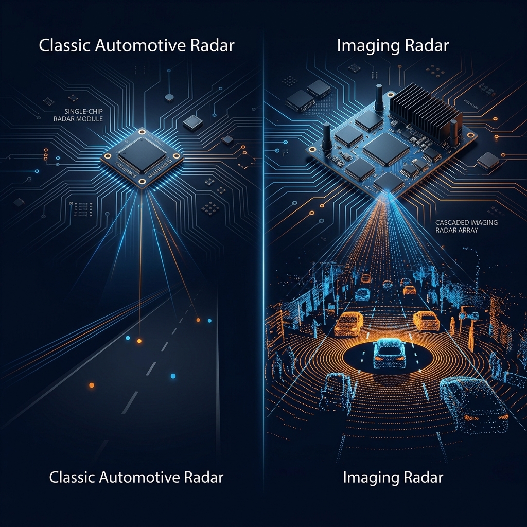
It’s worth being fair to the incumbent, because the incumbent earned its position. A typical classic automotive radar is built around a single MMIC with three transmit and four receive channels, giving twelve virtual channels through MIMO processing (CEVA). The FMCW waveform buys you excellent range and range-rate measurement regardless of channel count. What twelve virtual channels add on top of that is coarse azimuth and essentially no elevation. That sounds limiting until you remember what the sensor was asked to do. Adaptive cruise control, AEB against lead vehicles, blind spot detection, and cross traffic alert were the whole job. For those functions, range and Doppler carry most of the information, and the angular coarseness is tolerable.

Just as important is what the classic radar is architecturally, a smart sensor. Detection, clustering, tracking, and classification run inside the module, and what comes out is an object list (a few dozen tracked targets) over CAN. That design is self-contained in a way program managers learn to love. The sensor supplier owns the perception logic and delivers a validated black box. The OEM integrates a compact, well-understood interface. The data rate fits on a bus the vehicle already has, and the module’s power and thermal budget is small enough to hide behind a fascia without drama.

The weaknesses are equally well known, and they are exactly what pushed the industry toward imaging radar. With twelve virtual channels and no elevation, the sensor cannot reliably tell a stopped car in your lane from a manhole cover under it or an overhead gantry above it. All three are strong stationary returns at similar range and azimuth. The classic mitigation was to heavily de-weight stationary objects, which is precisely why stationary-vehicle scenarios have historically been hard for radar-based systems. Coarse azimuth also means two vehicles in adjacent lanes at similar speeds at 150 meters merge into one detection, since neither angle nor Doppler separates them. These aren’t implementation bugs. They are aperture physics. Fixing them requires more antennas, and more antennas is where the system-level story begins.

What imaging radar changes inside the box

Imaging radar attacks angular resolution by scaling the virtual array. Instead of one 3 TX / 4 RX MMIC, you cascade several transceivers into one coherent aperture. Texas Instruments’ four-chip AWR2243 cascade reference design forms 12 TX / 16 RX, giving 192 virtual channels (TI, TIDEP-01012), and Continental’s ARS540, generally cited as the first production-ready 4D imaging radar, uses a cascaded multi-transceiver architecture reaching the same 12 TX / 16 RX, 192-virtual-channel scale (Xilinx/Continental, EE Times). Purpose-built chipsets go further. Arbe’s platform forms 2,304 virtual channels from 48 TX / 48 RX, with a physical beamwidth around 1.25° in azimuth and 1.5° in elevation (Arbe). Add the wide sweep bandwidth available since regulators consolidated automotive radar into the 76–81 GHz band (FCC, 2017), and you get fine range resolution to go with the fine angles.

The functional payoff is real, and it holds up in field measurement. Elevation is the headline. Once the sensor can separate a return at bridge height from a return at bumper height, the stationary-object problem stops being a policy decision (“suppress stationary targets”) and becomes a measurement. Azimuth resolution around a degree separates adjacent-lane vehicles at range. And the output is no longer a curated object list. It’s a dense point cloud, hundreds to thousands of detections per cycle, that starts to look (squint a little) like a low-resolution lidar that works in fog.

During field benchmarking of candidate imaging radars (rain, fog, snow, the conditions where radar is supposed to earn its keep), the technology largely delivered on the detection side. But benchmarking sensors is the easy part. What follows is the part the datasheets don’t cover.

Change one: the interface, and with it, who owns perception

A classic radar’s object list fits comfortably on CAN. An imaging radar’s detection stream does not. Continental’s ARS548 RDI, for example, outputs its radar detections and objects over 100 Mbit/s automotive Ethernet at a 20 Hz cycle (AUMOVIO), and the interface definitions I’ve written for imaging radars have all been automotive Ethernet for data, with CAN relegated to diagnostics.

This looks like a wiring detail. It isn’t. The moment the sensor emits detections instead of objects, the tracking, classification, and fusion logic migrates out of the sensor and into central compute, and responsibility migrates with it. On a program where I was responsible for radar sourcing, the sensor data consumption and synchronization requirements shaped the central compute architecture directly, from how many Ethernet ports and switches it carried to how time synchronization was distributed and how much ingest bandwidth and memory the perception stack had to reserve per sensor. Multiply by every radar position needed for 360° coverage and the radar subsystem has become a networking and compute-budget problem before a single algorithm runs.

The program-level implication is that an imaging radar decision is really a compute-architecture decision. If your platform’s E/E architecture was sized around object lists on CAN, the radar upgrade drags the harness, the switch fabric, the time-sync design, and the perception software organization along with it. Budget for that in the architecture phase, not after supplier selection.

Change two: calibration becomes a bigger word

Each additional physical channel is another thing that varies with manufacturing tolerance and temperature. A cascaded multi-MMIC array must be phase-coherent across chips. The elevation axis you just bought must be aligned, not just the azimuth axis. And the mounting tolerance that was acceptable when your beamwidth was several degrees is not acceptable at one degree. Angular accuracy is only as good as your knowledge of where the boresight actually points.

Calibration therefore shows up twice, once in the supplier’s factory (array-level phase/amplitude calibration) and once on your vehicle line (end-of-line alignment). Both cost cycle time, floor space, and fixtures, and both are easy to underestimate when the program is still admiring point clouds. On one program, redesigning the radar calibration process and the associated manufacturing line procedure produced savings of approximately six figures, which tells you something about how much money was sitting in the original process. For high-channel-count radar, calibration turned out to be one of the main cost levers the program controlled, not a line item at the bottom of the integration plan.

So when you evaluate imaging radar suppliers, evaluate their calibration story with the same seriousness as their detection performance. Ask what is calibrated in their factory versus what your line must do, over what temperature range the calibration holds, and what the end-of-line procedure costs in seconds per vehicle. A sensor that needs a longer calibration station can erase its performance advantage in manufacturing economics.

Two more things live in this same blind spot. A sparse virtual array buys its narrow mainlobe at the cost of sidelobe level, so a dense point cloud can carry angle ghosts that your perception stack has to recognize and reject. Ask suppliers for measured sidelobe performance, not just the beamwidth headline. And time-division multiplexing across a dozen transmit channels divides the unambiguous velocity span, which matters the moment you care about fast closing rates. Both of those, plus mutual interference between high-bandwidth radars sharing a consolidated band, belong on the evaluation list next to detection range.

Change three: qualification risk rises with integration density

Nothing about imaging radar exempts it from automotive environmental requirements. The same −40 °C to +85 °C thermal cycling, vibration profiles, humidity exposure, and EMC/EMI validation I’ve defined for imaging radars apply to any radar behind a bumper. What changes is what’s inside the box while it endures all that: multiple MMICs instead of one, a larger and more layer-dense RF board, a substantial processor, and several watts more dissipation, often in the same fascia-concealed pocket with no airflow.

More power in the same enclosure means the thermal design works harder, and thermal margins are where radar RF performance quietly degrades. Transmit power, phase noise, and channel-to-channel coherence all care about temperature. And the calibration point from the previous section returns. It is not enough for the unit to survive temperature cycling. Its array calibration has to remain valid across the range. In my experience, module size, power consumption, and thermal footprint are exactly the parameters worth driving down with suppliers during BOM optimization, because they determine whether the same sensor can scale across vehicle architectures rather than being re-engineered per platform.

Put environmental and thermal qualification evidence on the critical path of supplier selection, not after it. A startup’s radar that dazzles in a demo vehicle has told you almost nothing about ten years and 150,000 miles behind a self-heating fascia in Phoenix.

Change four: the supplier conversation changes shape

Sourcing a classic radar is a mature exercise, with several Tier-1s carrying decades of field history, well-understood price curves, and an object-list interface that makes benchmarking straightforward. Running RFI/RFQ for imaging radar is a different conversation. The field mixes established Tier-1s with venture-backed startups. The chipset choices underneath (cascaded general-purpose transceivers versus purpose-built high-channel-count silicon) have real consequences for cost, power, and roadmap. And because the sensor no longer ships with the full perception stack, you are also buying an interface specification, a time-sync behavior, and a software integration burden that the datasheet understates.

My practical advice from those cycles is to decompose your vehicle-level requirements down to component-level radar requirements before the RFQ, with traceability, so that suppliers are bidding against your system’s needs rather than their sensor’s strengths. Field-benchmark candidates yourself under the weather conditions you’re buying radar for. And weight supplier viability and manufacturing maturity as hard requirements. An imaging radar startup’s five-year survival probability is part of your sourcing risk, because a mid-program supplier failure on a perception sensor is a program-resetting event.

Change five: the safety case moves with the processing

When a classic smart sensor mis-tracks a target, the failure sits largely within a supplier-validated black box, and the safety argument leans on the supplier’s evidence. When an imaging radar delivers detections and your central stack does the tracking and classification, the failure modes redistribute. The sensor owns detection-level integrity (and its calibration validity), while object-level errors belong to your perception software. Requirements decomposition has to reflect that split honestly. The L3/L4 component requirements you flow to the sensor supplier are now about detection probability, false-alarm density, latency, time-stamp accuracy, and calibration monitoring, not about “shall detect a pedestrian.”

The redistribution also changes what the architecture is entitled to claim. When radar could not separate a stopped vehicle from the gantry above it, the safety argument leaned on camera to carry stationary-object classification, and radar’s role in a degraded case stayed narrow. Elevation and finer azimuth make it defensible to ask radar to hold more of the stationary-object detection and overdrivability decision by itself. Classification in the camera’s sense is still not radar’s job, but deciding that a stationary return sits at bumper height and in lane no longer requires another sensor to confirm it. That question lands in the fusion and redundancy design. It sets what the vehicle is still permitted to do with a blinded or blocked camera, and how much of the fusion output any single sensor is allowed to originate. The counterweight is the false-positive budget, since multipath off guardrails and overhead structure still manufactures stationary ghosts that a denser array does not automatically remove. Those are allocation decisions, and they belong in the same requirements decomposition as the detection-level metrics above.

This is more work, but I’d argue it is also an opportunity. The redistribution puts the safety-relevant logic where the OEM or AV developer can inspect, test, and iterate on it, instead of behind a supplier’s IP wall. Regulatory pressure points the same way. FMVSS No. 127 is slated to require AEB, including pedestrian AEB that works in darkness, on US light vehicles from September 2029 (NHTSA). The rule has been under agency review and industry challenge since it was finalized. It doesn’t mandate any particular sensor, but higher performance floors in degraded conditions strengthen the case for radar that can resolve what it detects.

Change six: the data pipeline grows with the detections

A classic radar’s object list is a few dozen targets per cycle, small enough that logging it is an afterthought. You can log every radar on the vehicle for a full shift and think about the disk later. A detection stream breaks that habit. Hundreds to thousands of detections per cycle at 20 Hz, across four or five sensor positions, turns radar logging into its own engineering problem, bounded by what the logger can write without dropping frames, what the vehicle can carry, and how long an offload takes when the car comes back. Event-triggered logging helps, but only if the trigger already knows what is worth keeping, which on a new sensor is exactly what you don’t know yet.

The harder question is fidelity, and it follows directly from owning the tracker. You can only re-simulate what you stored, and once the tracker is yours, object lists stop being enough. Replaying or regression-testing that tracker requires the detections that fed it, even though object-level logs still earn their keep downstream for fusion and planning replay. Algorithm development pushes the other way, toward keeping something closer to raw, and that step is where the volume stops being a rounding error against the cameras and starts dominating the storage bill. Ground truth is the other half. Radar detections are not annotatable the way camera frames are, so usable labels generally come from association with another sensor, lidar most often, which means the labeling pipeline has to be built around cross-sensor alignment before it produces anything at all.

Choose your retention fidelity (raw, detections, or objects) at the same time you choose the sensor, and budget logging hardware, offload infrastructure, storage, and replay tooling as part of the radar decision rather than as a data-engineering surprise discovered during the first collection campaign.

Where classic radar still wins

A balanced accounting requires saying this plainly. For a large share of vehicles and functions, classic radar remains the right answer. Blind spot detection and cross traffic alert do not need 2,000 virtual channels. A corner radar’s job is served well by a small, cheap, single-MMIC module that sips power, needs no Ethernet port, and has a decade of field reliability behind it. The cost delta between a commodity corner radar and an imaging radar buys a lot of other content, and on a high-volume program that delta multiplied across sensor positions and a million vehicles is not a rounding error.

The honest framing is not “imaging radar replaces classic radar” but “imaging radar competes for the front long-range position on vehicles whose feature set justifies it, while classic radar keeps the corners and the value segments.” Trade studies I’ve run on radar technology roadmaps kept reaching versions of that conclusion: match the channel count to the function, not to the marketing.

What would change my mind

My position throughout this article has been that imaging radar is an architecture decision, not a sensor decision. It’s worth being explicit about what would soften it. If suppliers ship high-channel-count radars that emit a validated object list at acceptable latency over an interface the vehicle already has, the ownership argument in “Change one” largely dissolves. If end-of-line calibration for cascaded arrays becomes a solved procedure measured in seconds per vehicle, the cost lever I keep pointing at stops being much of a lever. And if in-vehicle networking and central compute get cheap enough that ingest budgets stop binding the architecture, most of the drag I’ve described goes with them. I haven’t seen those conditions on a program yet, but none of them is far-fetched, and a reader who has seen them should discount this article accordingly.

Until they arrive, the practical consequences hold. Size the E/E architecture for detection-level data before committing to the sensor, and pick the logging fidelity in the same breath. Decompose requirements to detection-level metrics so the redistributed safety case has something to trace to. And keep classic radar wherever the function doesn’t justify the channels.

The angular resolution line on the datasheet is real, and it solves real problems. I’ve watched it dissolve the stationary-object dilemma that haunted a decade of radar feature development. But the programs that succeed with imaging radar are the ones that price in everything attached to that line. The sensor is the easy part. It usually is.